H.E.S.S. Source Searches
Gamma-ray point sources observed by H.E.S.S. at TeV energies are candidate targets for this analysis. The scripts used to test for correlation with these sources are within the pev-photons/TeVCat directory.
Individual Source Tests
To fit each H.E.S.S. source location indiviually, run:
python individual_ts.py
This produces the file {prefix}/TeVCat/hess_sources_fit_results.npy, which stores the TS, \(n_s\), and \(\gamma\) for each source location. Convert these test statistics to pre-trial p-values with:
python hess_ts_to_pvalue.py
Note that this requires the unique declination background trials produce in the all_sky section. Add --use_original_trials to use the trials we generated instead. Finally, to calculate the sensitivity to each H.E.S.S. source at 1 PeV, given an unbroken power law with the best fit spectral index from H.E.S.S. data, run:
python hess_sensitivities.py --ncpu *desired_ncpu*
Combining the information from this section should give you results consistent with the following table:
| Source | \(\delta\) [\(^{\circ}\)] | \(\alpha\) [\(^{\circ}\)] | pre-trial p-value | \(n_s\) | \(\gamma\) | Sens. (x \(10^{-20}\)) |
|---|---|---|---|---|---|---|
| HESS J1356-645 | -64.50 | 209.00 | … | 0.0 | … | 3.72 |
| HESS J1507-622 | -62.35 | 226.72 | 0.29 | 2.5 | 1.3 | 4.75 |
| SNR G292.2-00.5 | -61.40 | 169.75 | 0.30 | 10.0 | 4.0 | 8.97 |
| Kookaburra (Rabbit) | -60.98 | 214.52 | 0.31 | 3.7 | 1.8 | 4.96 |
| HESS J1458-608 | -60.87 | 224.54 | 0.22 | 9.1 | 2.4 | 1.88 |
| HESS J1427-608 | -60.85 | 216.97 | 0.07 | 25.9 | 3.2 | 12.10 |
| Kookaburra (PWN) | -60.76 | 215.04 | 0.49 | 1.8 | 2.2 | 4.31 |
| SNR G318.2+00.1 | -59.47 | 224.44 | … | 0.0 | … | 7.79 |
| MSH 15-52 | -59.16 | 228.53 | 0.52 | 1.6 | 3.8 | 14.97 |
| HESS J1018-589 B | -58.93 | 154.74 | 0.07 | 23.7 | 4.0 | 4.75 |
| HESS J1018-589 A | -58.98 | 154.13 | 0.08 | 22.1 | 4.0 | 5.22 |
| HESS J1503-582 | -58.23 | 225.91 | 0.17 | 21.9 | 4.0 | 12.73 |
| HESS J1026-582 | -58.20 | 156.66 | 0.09 | 26.7 | 4.0 | 2.50 |
| HESS J1026-582 | -58.20 | 156.66 | 0.09 | 26.7 | 4.0 | 2.50 |
| Westerlund 2 | -57.79 | 155.85 | 0.08 | 32.0 | 4.0 | 9.35 |
| SNR G327.1-01.1 | -55.08 | 238.65 | … | 0.0 | … | 14.30 |
Stacking Test
Run the stacked likelihood test for all H.E.S.S. source combined by executing:
python stacking_test.py
The results are stored in {prefix}/TeVCat/stacking_fit_result.npy. To generate background trials use:
python stacking_test.py --bg_trials 100000 --ncpu *desired_ncpu*
The results should match the following table:
| Test Statistic | p-value | \(n_s\) | \(\gamma\) |
|---|---|---|---|
| 1.74 | 0.08 | 65.23 | 3.66 |
Skymap including H.E.S.S. Sources
To produce a plot of the all-sky scan p-value map with H.E.S.S. source positions overlaid run:
python plot_HESS_region.py
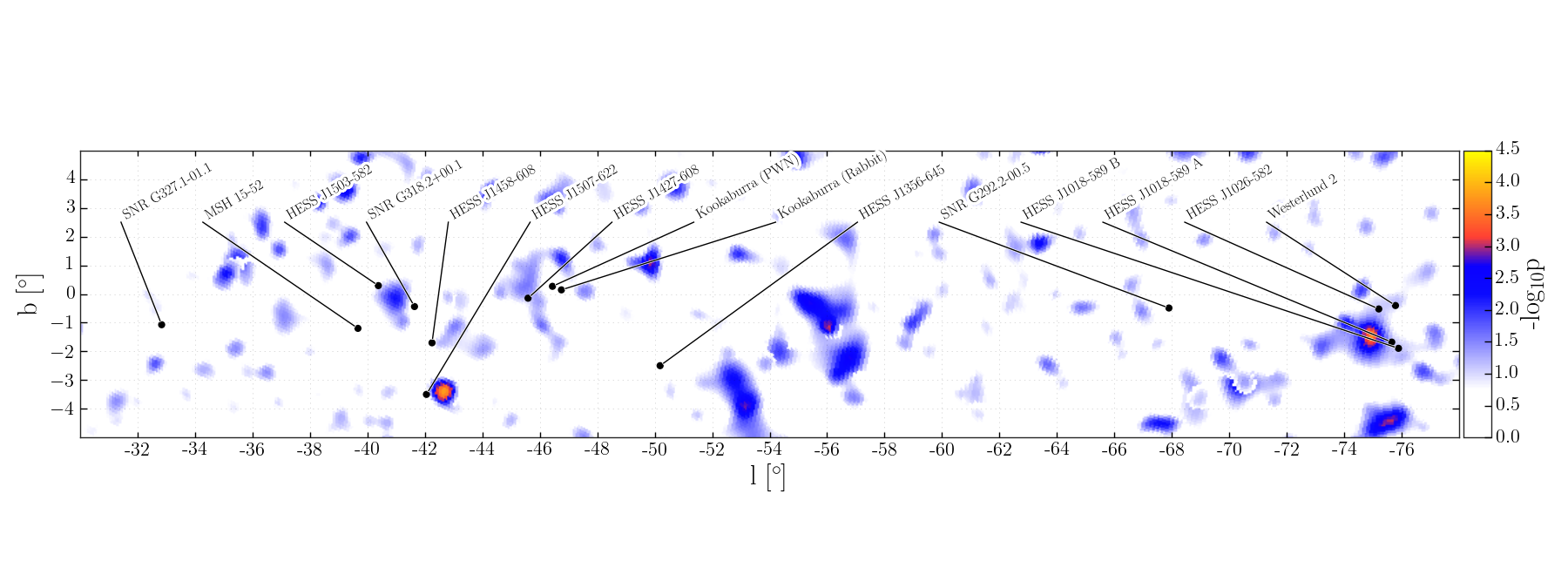
Figure 10: All-sky likelihood scan pre-trial p-value shown in galactic coordinates. The H.E.S.S. sources in the analysis field of view are shown in black.
Individual Source Limit
Plot best fit spectrum of H.E.S.S. J1356-645 compared to the IceCube upper limit with:
python plot_hess_sed.py
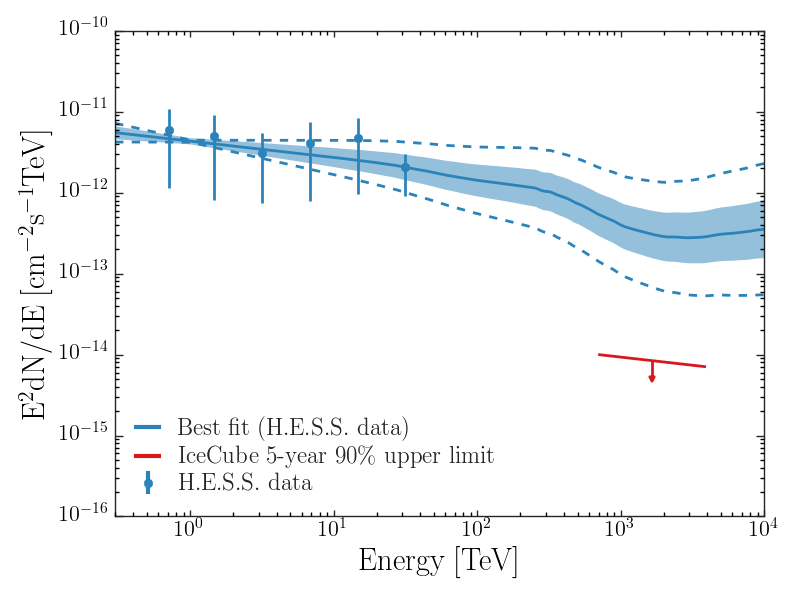
Figure 7 (right): Measurements of the source H.E.S.S. J1356-645. The best fit power law spectrum for the H.E.S.S. data is shown in blue. The shaded region denotes statistical uncertainty, while the systematic uncertainty is represented by the dashed lines. The 90% upper limit set by this analysis is shown in red.