Galactic Plane
The following scripts reproduce the section of the analysis which searches for diffuse emission from the galactic plane. All scripts are within the pev-photons/template directory.
Template Construction
To construct the template objects for each year of data, run:
python template_builder.py --year all
This creates a structured numpy array {prefix}/template/{year}/fermi_pi0_exp.npy with all the fields required by the template method.
To plot the Fermi \(\pi^0\) template convolved with detector acceptance (Figure 12 in the paper), execute:
python plot_template_x_acc.py
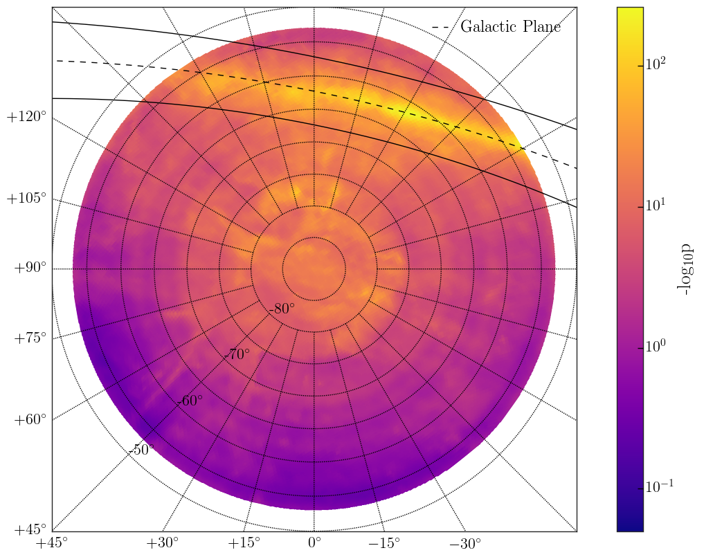
Figure 12: The Fermi-LAT \(\pi^0\) decay spatial template multiplied by the detector acceptance for the data year 2012.
Template Analysis
To run the likelihood test with the Fermi \(\pi^0\) template, execute:
python run_gp_analysis.py
This creates the structured numpy array {prefix}/template/fermi_pi0_fit_result.npy, which includes the test statistic and \(n_s\) values from the fit.
To produce a background trial test statistic ensemble, on submitter, run:
python cluster_bg_trials.py
The 10,000 trials produced are stored in {prefix}/template/trials/fermi_pi0. Then the p-value can be calculated via:
python p_value_calc.py
This adds the p-value to the fit results file created earlier. To skip generating your own trials, add the --use-original-trials option. Your result should match the following table:
| Test Statistic | p-value | \(n_s\) |
|---|---|---|
| 0.22 | 0.276 | 150.70 |
Sensitivity Calculation
To determine the sensitivity to the required level of precision (~1% uncertainty), we run signal injection trials on the cluster. First, we determine a reasonable range of injection points with:
python sensitivity_test.py
Which runs 100 trials per injection point. This step can be ommitted if you simply wish to compare final results. Next, we run 10,000 trials at each injection points on the cluster. On submitter, execute:
python cluster_sens_trials.py
Finally, perform a \(\chi^2\) fit on the fraction of trials above 0 as a function of the number of injected events with:
python sens_fit.py
This yields the \(n_s\) value which corresponds to a fraction of trials above 0 at 0.90 with 1% precision and calculates the corresponding flux. The output (stored at {prefix}/template/fermi_pi0_sens.npy, should match the following table:
| \(n_s\) | \(n_s\) error | Flux [\(GeV^{−1}cm^{-2}s^{-1}\)] | Flux error |
|---|---|---|---|
| 491.2 | 2.3 | 2.63e-22 | 1.23e-24 |
Plots
To produce a plot with ARGO-YBJ, CASA-MIA, IC-40, and IC-86 fields-of-view overlaid on the Fermi \(\pi^0\) skymap (figure 13(left) in the paper), run:
python plot_fov.py
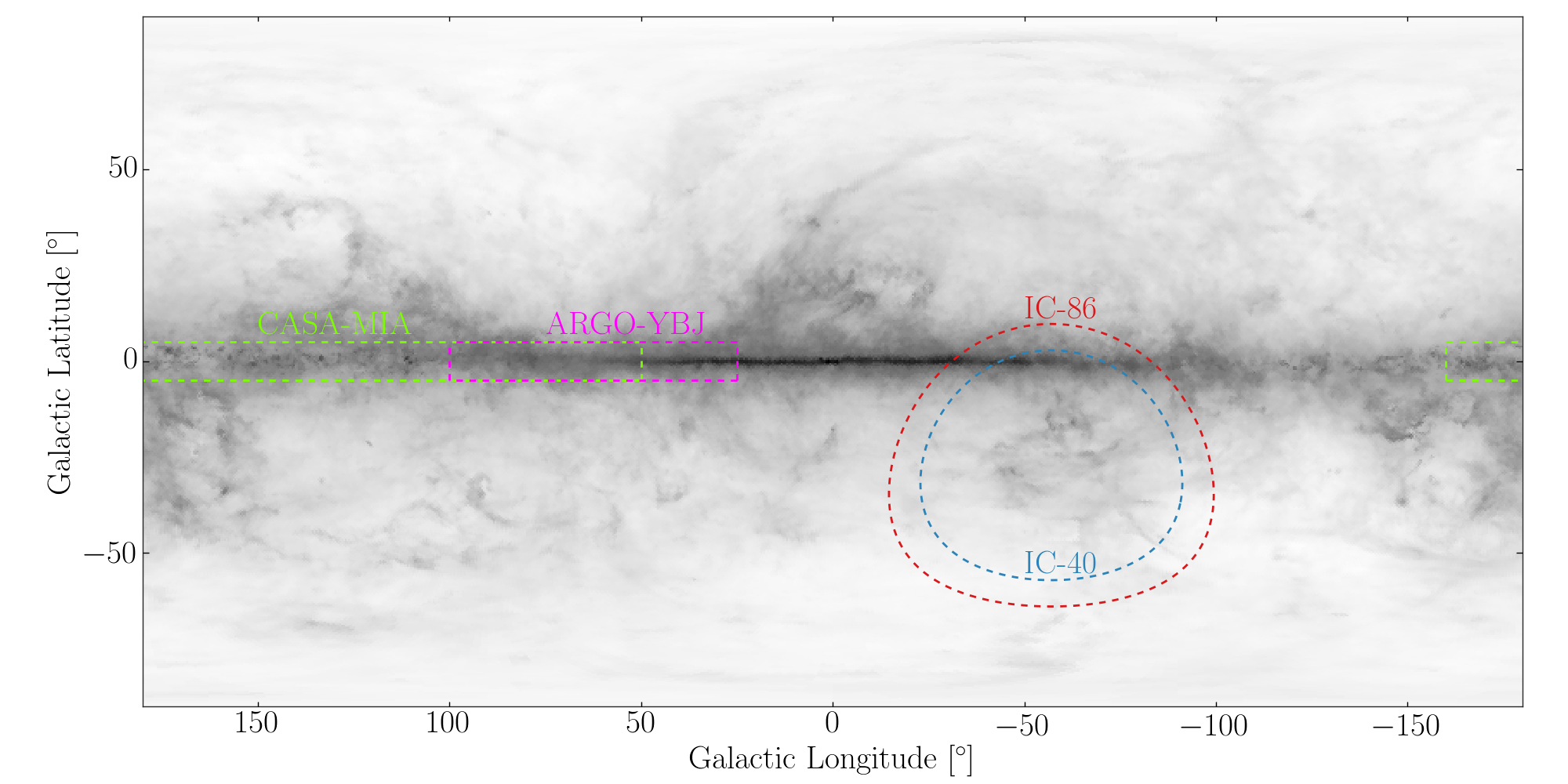
Figure 13 (left): The respective field of views of CASA-MIA, ARGO-YBJ, IC-40, and this analysis overlaid on a map of the \(\pi^0\) decay component of the Fermi-LAT galactic plane diffuse emission model.
To produce the plot comparing upper limits on the normalization of the Fermi pi0 decay emission model (figure 13(right) in the paper), run:
python plot_galactic_limit.py --fermi_limit
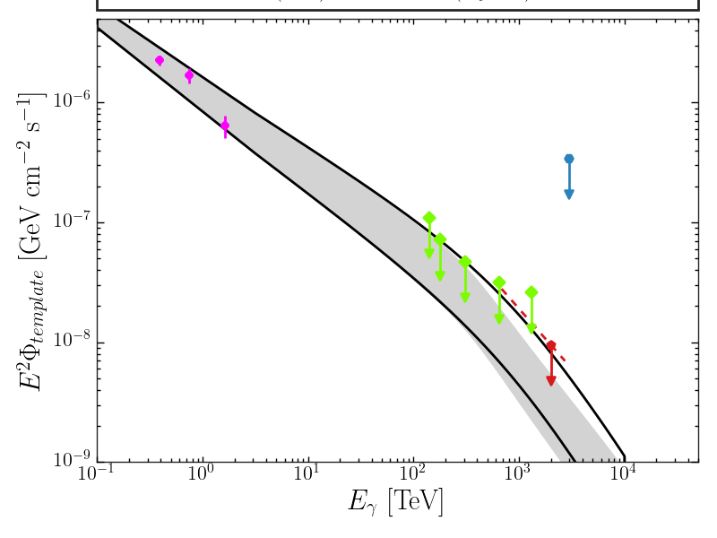
Figure 13 (right): The IceCube 90% confidence level upper limit on the flux from the \(\pi^0\) decay component of the Fermi-LAT galactic plane diffuse emission model in our field of view as compared to results from ARGO-YBJ, CASA-MIA, and IC-40. Dotted lines show the E \(^{-3.0}\) spectrum, used for obtaining IceCube upper limits, over the energy range containing 5% to 95% events in the final sample. Also shown are unattenuated and attenuated flux predictions from Vernetto 2017.